Data Structures - Trees
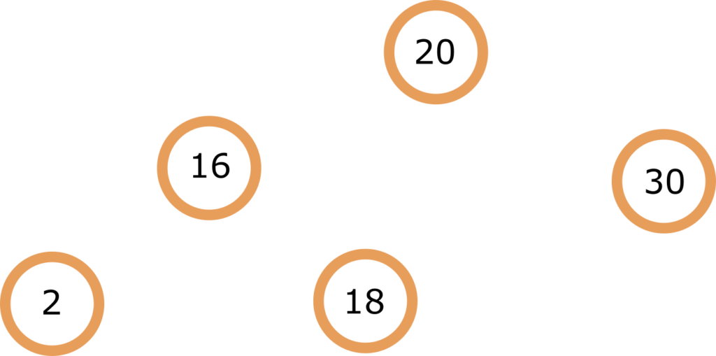
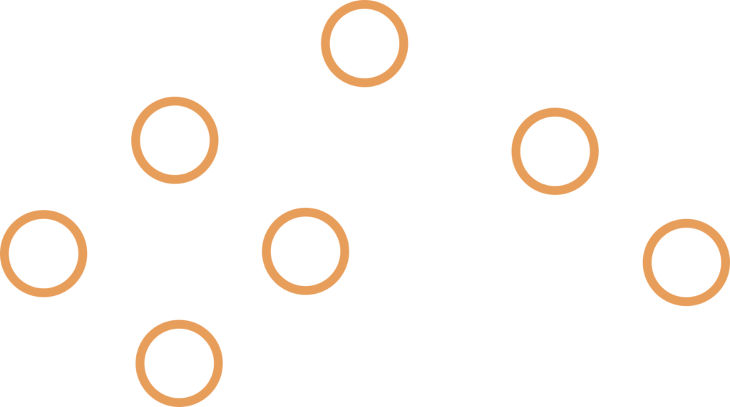
Up until this point we looked at only linear data structures. Now it’s time for trees, which are a hierarchical. This means that the elements contained in the tree are in a hierarchy and each element can have multiple subordinate elements. They are used all over the web, html code is basically a tree structure, comments on social media are trees, folders are trees… Trees are also used because of their optimized search and manipulation in sorted data bases. Trees have been used in multi-stage decision-making ( before neural networks came to the party ). Trees are, as linked lists, dynamic data structure so they support insertion and deletion of elements. What makes them more desirable than linked lists or array is their time complexity, O(log N) for search, insertion and deletion in something called a balanced binary search tree but more on that later. To make things a bit more clear here is the tree terminology in visual:
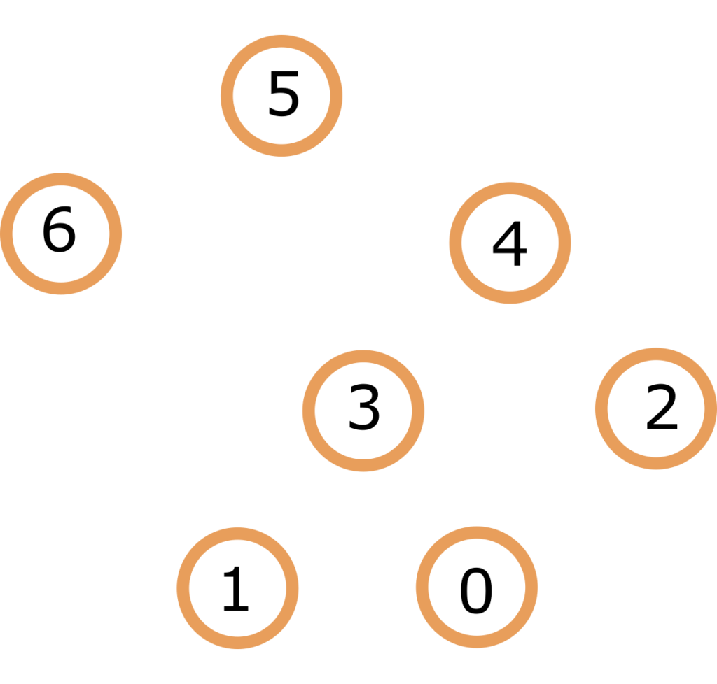
So the elements of the tree are, as with the Linked Lists, called nodes. Top most node is called root of tree. Nodes are in child – parent relationship, one node can have multiple children but only one parent, nodes that have no children are called leaves.
Binary Tree
This is type of tree that comes up when you usually talk trees in data science. In a binary tree each node can have up to two children, these are called left and right child. Tree is represented by the root node, same concept as linked lists. Here is how the definition of a binary tree node would look like in C++:
class BTNode
{
		int data;
		BTNode* left;
		BTNode* right;
}
So as you can see it’s pretty simple and straight forward. Where things get interesting in trees and graphs are in traversal, insertion and deletion of elements. But we’ll cover tree traversal in the algorithm course, for now let’s take a look at some properties of binary trees and some other types of trees.
Binary tree subtypes and properties
Before going over some facts about BTs we need to know different subtypes.
- Perfect binary tree – all levels are complete, the most optimal for traversal, insertion/deletion and manipulation of data
2. Full Binary Tree – all nodes have 0 or 2 children
3. Complete Binary Tree – all levels are filled, or all nodes in last level are as left as possible
4. Binary Search Tree ( BST )- left children are smaller than the parent, right are larger
5. Balanced BT – O(log N) height where N is number of nodes, examples are AVL trees and Red Black Trees ( we’ll talk about them later ), they balance the height and number of nodes to maintain the O(log N) height, these are, after the perfect binary trees, the most performant
6. Unbalanced ( degenerate ) BT – example is similar to linked lists, most if not all nodes have one child and traversal and all other operations are the worst case scenario O(N) complexity
Now that we know all the forms BT can have let’s talk on properties, most are useful only in perfect, full and complete BTs.
- Maximum number of nodes at level i of a BT is 2i — this considers the root node being the level 0, level underneath the root has 2 node ( two children of the root ) or 21, level after that 4 ( 2 children from each of nodes from the last level, so 22. If the tree is a perfect BT number of nodes at level i is equal to 2i.
- In a BT with height/number of levels of h number of nodes is max 2h-1 — this considers root as height of 1, again maximum number is achieved when BT is perfect. You can think of number of nodes in BT as sum of all levels, and number of nodes in a level is 2i for each level i so number of nodes is the sum 1 + 2 + 4… + 2h and that sequence is equal to 2h – 1;
- If BT is full, number of leaves is equal to number of nodes with 2 children + 1 — to proof this, 2h-1 – number of leaves, N – number of internal nodes, and 2h – 1 as number of all nodes, N is the difference between all nodes and leaf nodes so N = 2h-1 – 2h – 1 = 2h-1 * ( 2 – 1) – 1 = 2h-1 – 1, because number of leaves is 2h-1 ⇒ number of leaves = N + 1
ALV and Red Black Trees
We’ll just cover the basic concepts of there two types of binary trees because I could go on and write a post about just inserting elements into one so I’ll keep things simple. These two trees are what is called self balancing trees.
AVL trees use rotation method on insertion and deletion to keep the difference between height of left and right subtree of every node less than or equal to 1.
Red Black trees along with the data on each node store a 1 bit of colour, either red or black. Balance is kept with the rule that two red nodes cannot be adjacent, aka red node cannot have a red child or a red parent. Also all leaf nodes are black and root is black.
These trees exist because they keep the operations on the tree in O(log N) time, which is the case with BST in general but the worst case can have O(N) time if the tree height gets to high in comparison to number of nodes.
Red and black trees are used in implementation of C++ and Java maps and sets, Linux CPU scheduling and in K-means clustering algorithms and computational geometry. In general if your program requires large number of insertion and deletion RB trees are better than AVL trees
AVL trees are also used to implement maps and dictionaries and also in large data bases where there isn’t a lot of insertion and deletion but frequent searching.
This was mostly a theoretical introduction to trees, where trees get practical are in the algorithms for traversing and manipulating data stored in them. Those topics will be covered in a course on algorithms that’s coming soon.